daily

2026-09-10
1

Enniscorthy Blackstairs Blues weekend

Wexford Local · original → · 8/10 · Local Wexford: Enniscorthy Blackstairs Blues Festival this weekend
[image →]Holohans where many Blackstairs Bues acts are taking place this weekend. (Pic; WexfordLocal.com) By Dan Walsh The 33rd Blackstairs Blues Festival brings a musical atmosphere to Enniscorthy…
[image →]
Holohans where many Blackstairs Bues acts are taking place this weekend. (Pic; WexfordLocal.com)

By Dan Walsh

The 33rd Blackstairs Blues Festival brings a musical atmosphere to Enniscorthy this weekend kicking off at 6.30pm on Friday with Garry Cogdell (USA) and Dermot Byrne playing at Stamps in Market Square.

Free sessions will then take place in Dawsons, Rackards, Treacy’s Hotel, Holohans, The Antique Tavern, Riverside Park Hotel, the IFA Centre and The Bailey, with fringe events at Enniscorthy Library and the Athenaeum Hall. The weekend concludes on Monday at 8.30pm with a Survivors Gig by Austin Walkin Cane and the BC Blues Band in Holohans.

According to a spokesperson; “the festival will feature a massive variety of styles, from intimate acoustic sessions and traditional Chicago blues to high-energy blues-rock performances hosted across local pubs, hotel stages, and community venues.”

First established in 1995, the event holds a legendary place on the Irish music calendar as Ireland’s longest continuously running blues festival. What started as a modest gathering in Bobbie Rackard’s pub on Rafter Street has grown into a landmark regional event, taking over the entire town every September.

The festival is backed by the Enniscorthy Municipal District providing €2,500 thanks to the Arts Office Small Arts festival Fund and Fáilte Ireland Festival Scheme.

The full programme of events is available at all venues and other outlets in Enniscorthy and on the Blues Ireland website.

2

GPT-6 Astra, looped transformers, and hidden reasoning

Hacker News · original → · 8/10 · AI: GPT-6 Astra analysis, looped transformers, reasoning architecture
A lot has happened in the last few weeks. I am sure that OpenAI’s GPT-6 Astra is top of mind for everyone right now. In particular, thoughts on its performance, the looped transformer/recurrent…

A lot has happened in the last few weeks. I am sure that OpenAI’s GPT-6 Astra is top of mind for everyone right now. In particular, thoughts on its performance, the looped transformer/recurrent depth aspects, and rumors that Astra is “hiding” its reasoning trace (i.e., chain of thought). So, in this article, I want to start with some brief impressions of Astra and some thoughts on where all this is headed. Then, I will discuss, in detail, what “looped transformers” are, and how (or rather, if) this relates to hiding chains of thought. Lastly, after covering the basics of the looped transformer, I wanted to highlight some new insights from recent research papers on the topic. 1. GPT-6 Astra impressions First things first. Before getting into the architecture rumors and related research literature, let me briefly summarize some GPT-6 Astra observations and tidbits. Last week, OpenAI’s new GPT-6 Astra was released with a big fanfare. I used it over the past couple of days, and it’s an exceptionally good model, likely the best I’ve used as of this writing. But what, exactly, has it improved, and how? 1.1 Astra benchmarks Astra is the best model I’ve used so far, and it’s disproportionately good at 3D rendering and animation tasks (relative to other models). With that, I mean that while it leapfrogs its GPT-5.6 predecessor in practically all categories (writing, math, coding, and more), it especially does so when it comes to graphical demos. We can see this also reflected in the benchmarks. For instance, GPT-6 Astra is really good at math and coding, as shown below. One of the highlights (not shown in the figure) is that Astra also achieves 99.9% on the ARC-AGI-3 benchmark (GPT-5.6 Sol only 7.8%), which measures a mix of solving logic puzzles and generalization. However, the math, coding, and computer use benchmarks are more interesting because they are closer to real-world use. Coming back to the Artificial Analysis Coding Agent Index v1.4 (lower right in the previous figure), which blends several agentic coding tasks, GPT-6 Astra is clearly at the frontier, but it doesn’t pull ahead by leaps and bounds. This can also be seen in the general Artificial Analysis Intelligence Index shown below, which blends different types of tasks, not just coding tasks. Now, the big advantage of Artificial Analysis benchmarks is that they are independent and thus may be a bit more trustworthy than self-evaluated benchmarks by model developers. The harness setup depends on the benchmark. For example, GDPval-AA and AA-Briefcase use their open-source, minimal Stirrup harness across the different LLMs they compare. In the Intelligence Index v4.2 shown above, Terminal-Bench v2.1 uses Terminus 2, and τ³-Banking uses the τ-Bench harness. The separate Coding Agent Index also compares different coding-agent harnesses. For evaluations that use a shared harness, this makes it more of an apples-to-apples comparison. At the same time, during model training, models are typically developed with one primary harness in mind (and fine-tuned less on other harnesses). Plus, the primary harness is often developed to suit and amplify a model’s strengths. So, some of the agentic evaluations might underestimate how well Astra performs in its primary harness. How much this affects its Intelligence Index score would need to be tested by comparing Astra across harnesses on the same tasks. As a side note, as a colleague recently suggested to me (as also recommended by the Claude Code lead), it’s maybe not a bad idea to delete (/archive) some of your existing AGENTS.md contents and SKILL.md files, as newer LLMs have become more efficient at understanding the prompt and solving the problem at hand. The extra hand-holding could unnecessarily constrain newer models and lead to worse solutions. Of course, I am not suggesting never using SKILL.md files again, but for some workflows, because they can improve efficiency upon reuse, since the model doesn’t have to rediscover them. But what I am suggesting is that some workflows don’t need describing, and “old” descriptions may no longer be ideal, and the LLM may be able to come up with better solutions. So, it’s perhaps time to update or regenerate said instruction files. 1.2 Computer use capabilities GPT-6 Astra seems to be exceptionally strong in image and rendering tasks. When these tasks involve interacting with graphical user interfaces, they also demonstrate computer-use capabilities, meaning the model operates software on your local computer through the Codex/ChatGPT app. Computer use is where the model really shines compared to others, and anything graphic-related also makes for interesting and intuitive demos on social media platforms. There are tons of examples of impressive demos out there, from modeling rendering New York City in blender to virtual open house tours. To pick one example, below is a comparison where I had GPT-6 Astra Medium and High redraw a picture of me in a browser version of MS Paint using the mouse on my computer (not Extra High and Max, because I didn’t want to waste all my tokens :)). This highlights not only the model’s artistic capabilities but, more importantly, its ability to use tools on one’s computer (in this case, Paint; you can see the model using the interface via the mouse cursor). This is not the first model that, inside a harness, is capable of general computer use. For example, I successfully used GPT models for some UI tasks (e.g., expense-related tasks in Excel) and so on since earlier this year. However, computer use is a relatively new capability, enabled by the harness, and usually feels not quite as mature yet. This makes sense. LLMs are text models, so naturally the lower-hanging fruit is writing and coding and using APIs and CLIs. At the same time, there are many tools and software that don’t expose CLIs (yet), and instead of waiting until someone designs that interface, why not improve models to use graphical user interfaces (and, as mentioned before, this makes for pretty and impressive demos, anyway)? This is somewhat analogous to the emerging humanoid robot developments. Sure, humanoid robots are not the most efficient robots, for example, at the assembly line, where special-purpose machines exist. But they are versatile. So, I expect the upcoming months (or years) also to be an era of computer use refinement on both the LLM and the agent harness layer. I.e., in addition to the current capabilities, and expanding their math and coding capabilities, models will be trained with an increasing amount of computer use in mind. And this will also make LLMs more accessible for everyday computer tasks outside the tech world (”Hey ChatGPT, please do my tax return” :)) 1.3 Computer use training The computer usage trend is also consistent with the recent reporting that OpenAI purchased tens of thousands of Mac Minis and Mac Studios for Reinforcement Learning. So, here the Macs are not used to literally train the models (it’s better to use GPUs for that) but rather to expose macOS during the model training for the model to learn to use said operating system and the tools therein. So, how does computer-use training on said Macs work? In short, the Macs (or their macOS operating system, to be precise) serve as an environment that the model can interact with during training. The basic workflow looks like this: Prompt the model by giving it a task, such as “open an app xyz and do abc”. Provide it with screenshots of the macOS interface (this is usually done by the harness). The LLM then predicts mouse/keyboard actions (click, key presses, scrolling, and so on). Execute those actions on the Mac (again, this is done by the harness). Feed new screenshots of the updated environment after performing the actions in the previous step. Repeat steps 2-5 until the task succeeds or fails. Use success/failure signals and verifiers (or graders) as training feedback, including reinforcement learning during post-training; this is analogous to regular Reinforcement Learning with Verifiable Rewards (RLVR). Again, the Mac is mostly the environment here and not the machine for running or updating the model during training. The model likely sits on NVIDIA GPUs and is fed via API to said Mac. By the way, NVIDIA’s CEO mentioned that GPT-6 Astra was being trained on ~100,000 Grace Blackwell GPUs. 1.4 GPT-6 Astra is still a reasoning model The focus on computer-use training discussed in the previous section is not a fundamental paradigm shift in the training pipeline. GPT-6 Astra (and likely any LLM in the foreseeable future) is still a reasoning model. This means the LLM is trained with reinforcement learning with verifiable rewards (RLVR) and produces intermediate reasoning traces (chains of thought) But I will discuss the reasoning model aspects of GPT-6 Astra (especially regarding hiding chains of thought) a bit later in this article. 2. Looped transformers That being said, about two days before the official model, the news magazine The Information published an articlereporting that, according to some inside information, Astra is using a concept called “recurrent depth” or “looped transformers.” Since LLM architectures are within my area of expertise and my passion, I created a short lecture video explaining the general looped transformer mechanism and addressing the comment about hidden reasoning chains, which you can find below. In the following subsections, I’ll first explain what looped transformers are, and I’ll revisit the comment about the hidden chains of thought later in this article. (The looped transformer explanation may seem a bit long, but I really think that it helps with establishing a foundational understanding of the technique, which is then useful to judging the claim that it obscures the reasoning traces or chains of thought.) 2.1 Reusing transformer blocks So, what’s a looped transformer? A Looped Transformer is essentially an architectural tweak, with the main idea being to pass the intermediate representations through the same transformer blocks multiple times (instead of just once). Compared to just adding more blocks, the “trick” here is that the weights stay the same across these passes. Definitions & Jargon Throughout this article, I’ll use the following terms: A transformer block is a unit containing attention, a feedforward module, normalization, and shortcut connections. These blocks are often called “transformer layers” in papers. A stack is a sequence of transformer blocks. A block application means running an input through a transformer block once. The looped transformer is nothing new, and the basic idea already appeared in the Universal Transformers paper from 2018. But before discussing Universal Transformer, let’s start with a simpler example, Nanbeige4.2-3B, a recent open-weight LLM that came out in July and that I covered on Substack Notes and in my LLM Architecture Gallery earlier this summer. The Nanbeige architecture, shown below, essentially looks like a regular transformer. However, notice that it has an extra (orange) arrow looping back to the beginning of the transformer stack. Let’s walk through this from the bottom up. First, as in any other transformer-based LLM, the input text is tokenized and converted into embedding vectors. These vectors then pass through 22 transformer blocks, and each of these 22 blocks has its own weights. However, the looping transformer aspect here is that after the first pass, the hidden states are fed back through the same 22 blocks. So, block 1 is applied again, followed by block 2, and so on up to block 22. If we were to unroll this computation, we would have 44 transformer block applications. However, compared to a conventional transformer with 44 distinct blocks, the second stack of 22 block applications reuses the weights from the first stack. For example, block application 23 uses the weights of block 1, block application 24 uses the weights of block 2, and so on. So, the whole idea here is that we increase the effective depth from 22 to 44 block applications without adding another set of transformer weights. By the way, why 2 rounds, not 3, 4, or more? There are not many details in the Nanbeige paper, but they say that this was essentially the most efficient setup. Increasing the loops from 2 to 3 can increase modeling performance, but the extra computational cost wasn’t worth it. 2.2 Looping costs So, why would we do this looping in general? This is essentially an alternative to just making the model bigger by adding more transformer blocks. So, for instance, a model that uses 22 transformer blocks twice has roughly half as many (transformer-block) parameters compared to a model with 44 conventional blocks. This then reduces the memory needed to store the weights. As a side note, note that the embedding and output layers, which are usually large and make up a substantial portion of the total, are separate from this comparison. (In the case of Nanbeige 4.2 3B, the embedding and output layers make up ~25% of the total 3B parameters; with weight sharing between those two, we could reduce that to 12.5%.) Of course, reusing the same blocks in a loop still requires computation. More precisely, we pass the intermediate inputs through 44 block applications during the forward pass. And, during training, gradients flow backward through both repetitions of the shared stack. So, compared to using the 22 blocks only once, this adds substantial work. Actually, it’s similarly expensive as having 44 distinct blocks (except the optimizer has fewer distinct parameters to update; backprop still runs through all 44 block applications). There is also the KV cache, which stores the attention keys and values of previous tokens for reuse in conventional and looped transformers in each next-token generation step. By the way, I have a standalone article on KV caching here if useful: But back to the topic. Even though there is weight-sharing in looped transformers, the intermediate states that enter a block are different on the second pass. Consequently, in KV caching, the resulting keys and values are also different between these two transformer stacks (just like in the no-looping case). So, there are no KV cache-related savings either. To make this more concrete, for example, consider block applications 1 and 23, which both use block 1 in the looped transformer setup. But each application still needs its own KV cache entries. So, since we have to keep separate caches for both passes, the repeated stack of 22 blocks has the same KV cache requirements as a conventional transformer with 44 distinct blocks. Interestingly, the Nanbeige researchers reported in the paper that they tried sharing the KV cache between passes. This, of course, halved the KV cache size, but the model performed worse than the version with separate caches (which is the version they released). Just to complete the Nanbeige discussion before moving on and looking at some other looped transformer designs, their technical report also discusses two other choices or trade-offs. Training the looped architecture from scratch worked better than converting an already pre-trained transformer through upcycling. And two passes gave their preferred trade-off, as mentioned in the previous section. More passes brought only small additional gains while slowing training and making optimization less stable. So, the number of passes is another architectural choice we have to make. As mentioned before, in Nanbeige, this is fixed at two. But we can also make it depend on the token, as we will see next. 2.3 Universal Transformers and flexible loop counts Now, let’s come back to Universal Transformers. In Nanbeige, we apply a stack of 22 transformer blocks twice. In the Universal Transformer paper from 2018, we repeatedly apply the same transformer block instead of repeating a stack of transformer blocks. The main idea is similar, though. Also, the number of steps can be fixed, but the paper also explores adaptive halting. For example, a token at a particular position may only go through one or two loops. Another may go through three or four loops, and so on. This gives the model flexibility to allocate the compute to those tokens that benefit from extra computation. How is the looping number decided? Here, the model uses a small, trained function that outputs a so-called halting probability for each position at each step. It adds up these probabilities over these successive loops and then stops looping at a given position once the sum exceeds a threshold value. In addition, a maximum loop count also limits the computation just in case. Another example of a looped transformer is ByteDance’s Ouro, which I also covered in my LLM Architecture Gallery. For instance, Ouro-Thinking 2.6B applies the same stack of 48 transformer blocks four times. That’s 192 block applications while storing weights for 48 distinct blocks. Basically, that’s a more extreme case than Nanbeige. Additionally, a learned exit gate assigns probabilities to the different exits, and a threshold on the cumulative probability determines which pass supplies the output. So, it’s also borrowing the adaptive halting idea from Universal Transformer, which Nanbeige didn’t use. (However, there is a practical caveat here. The released Hugging Face implementation computes all configured passes before selecting an output, so it seems like the number of loops is effectively hard-coded to 4). 2.4 Routing flexible loop counts Another approach is Mixture-of-Recursions, a paper from 2025 that is essentially a more sophisticated version of the Universal Transformer discussed earlier. Similar to the Universal Transformer, individual tokens pass the transformer blocks one or more times as illustrated in the figure below. However, the innovation is how this looping number is determined on a per-token basis. In the following figure from the paper, the looped (repeated) stack is called a recursion block here. This contains several transformer blocks, and it sits between separate first and last transformer blocks (labeled Layer 0 and Layer L-1). How does the model decide how many times a token should go through the recursion block? In the previously discussed Universal Transformer, it’s based on a learned halting probability at each step. This Mixture-of-Recursion approach here uses a small, learned router. This is similar to the routing idea in a mixture-of-experts model, except that here the routing decision determines how many times to apply the shared stack. The router operates on a token’s hidden representation, which also contains information about its context. So, we shouldn’t think of this as assigning every occurrence of a particular token the same number of passes (i.e., the word “People” in the figure above doesn’t always go through a loop of 3). The decision can change depending on where that word appears and what came before it. Now, how does the routing work exactly? The paper explores two ways to make this routing decision, as illustrated below. In expert-choice routing, which is shown in the left subpanel in the figure above, each recursion step selects which tokens it will process. Tokens that exit are excluded from later steps. In token-choice routing, shown on the right, the router makes one decision at the beginning, assigning each token to a path with one, two, or three passes. In both cases, the transformer weights are reused across passes, similar to Nanbeige, etc. But the additional flexibility comes from choosing how much computation each token receives. The model and its routers are trained together, so the model learns to work with these different paths during training. 2.5 How well does this work? The plot from the Mixture-of-Recursions paper below compares a regular transformer (Vanilla), a transformer with fixed recursion (Recursive), and Mixture-of-Recursions (MoR) for different model sizes and compute budgets (x-axis). At the smallest model scale, the regular transformer performs best. For the larger models, Mixture-of-Recursions catches up and often performs better, especially at the smaller training budgets. At the largest budget, several of the curves are very close. So, the advantage depends on the model size and how much compute we spend on training. Another detail here is that equal training compute doesn’t necessarily mean an equal number of training tokens. By skipping some computation, Mixture-of-Recursions can process more tokens within the same budget. I think this is an interesting example because it shows that there are several choices within the looped-transformer idea, that is, how many loops there are at each position and how that’s decided. So, in short, we can say that using looped transformers can improve model quality at a fixed compute budget if the model is large enough. (It also illustrates the importance of running some experiments at scale; e.g., just looking at the smaller 135M parameter model, we would have drawn the opposite conclusion.) 3. Side note: Recurrent Neural Networks (RNNs) By the way, if you have a background in deep learning (or even artificial neural networks in the 1990s), the looping or “recurrent depth” idea should be somewhat familiar. Remember recurrent neural networks (RNNs)? The whole idea in RNNs is to reuse the layers (weights) from a previous iteration. The main distinction is that RNNs reuse their weights across time steps. That is, the hidden state is carried forward from one token to the next. In the looped transformer, the looping of a token is across the architecture depth. Or, in other words, in a conventional RNN, each step takes the next element in the input sequence and the hidden state from the previous step. So, when the RNN is processing a chunk of text, it reads one word or token at a time and carries information from the earlier words forward in its hidden state. In a looped transformer, the intermediate representation of a given token goes through the transformer stack multiple times. The model still uses attention to pass information between tokens. If this analogy is a bit too confusing, don’t worry about it too much. A perhaps simpler way to think about looped transformers is to think of them as reusing transformer blocks, similar to making the model bigger but with weight sharing. 4. Does Astra even use looped transformers? Before we discuss whether the looped transformer mechanism obscured reasoning traces, as rumored in The Information quote from earlier, does GPT-6 Astra even use the looped transformer concepts? We have to keep in mind that this is still just a rumor or scoop, with no official confirmation. If the model were open-weight, we could double-check this ourselves, of course, but in this case we have to rely on unverified reporting. However, I think it’s highly likely that GPT-6 Astra uses looped transformer aspects. First, there is the reporting mentioned above. Second, it’s a technique that has shown promise in past studies (as discussed earlier), so why not? Third, OpenAI’s chief scientist said the following. [...] The depth of the computation graph for our present frontier models, including Astra, is within a factor of two of GPT-4. [...] However, this doesn’t confirm the looped transformer architecture explicitly, and it could also just mean they use twice as many regular transformer blocks. In my opinion, the success (i.e., good modeling performance) behind Astra is likely primarily due to other reasons, namely improved training recipes and training data. The looped transformer tweak might help a bit, but I think that The Information is overestimating its contribution. 5. Hiding chains of thought Next, let’s finally address the elephant in the room: does looped transformer obscure the reasoning traces? First, OpenAI has been hiding (most of) the reasoning traces from users from the very beginning, since OpenAI o1, anyway. So, for the end-user, there shouldn’t be a big difference. So, the interpretation-concern is mostly with respect to the model developers. Either way, I don’t think that looped transformers are significant contributors towards hiding or obscuring chains of thought. To explain my own reasoning (no pun intended), let’s take a step back and explain how reasoning models work. 5.1 Reasoning in brief Reasoning models typically generate intermediate steps before producing a final answer. These steps use regular text token (that are optionally hidden from the user in some user interfaces) and called a reasoning trace or chain of thought. For example, say we ask for two numbers whose sum is 10 and whose product is 21. In the figure below, the model tries 5 and 5 at first. While the sum is correct, the product is 25, not 21. Next, it then tries 3 and 7 and checks both conditions again. The figure illustrates how a reasoning model “reasons,” including backtracking. That is, the model notices a mistake, then revisits an earlier choice, and then continues with a different approach. Note that the model still generates one token at a time, using the prompt and previous tokens as context. So, these intermediate steps work as a scratch pad and add computation before the final answer. The final answer can then be much shorter than the reasoning trace that preceded it, as shown in the example above. (OpenAI tends to hide most of the reasoning traces from the users.) For more details on understanding and developing reasoning models, I recommend my book Build a Reasoning Model From Scratch. 5.2 Token usage and shorter chains of thought Now, extra tokens in the reasoning trace add more computation. Looped transformers add more computation, because the tokens go through more transformer blocks. One might argue that a model with looping uses more computation internally, it doesn’t need as many external thinking tokens. Below is a selection of the GPT-6 benchmarks with the output token number on the x-axis. We can see that GPT-6 Astra doesn’t necessarily use fewer tokens than its GPT 5.6 Sol predecessor across effort levels overall. However, at a fixed accuray, it is true that GPT-6 Astra uses fewer tokens than GPT 5.6 Sol. Is this a concern for interpretability? Not necessarily. Using fewer tokens could just mean that the model is more capable and makes fewer mistakes, uses less backtracking, and so on. I.e., it might just get more things right on the first try. To me, that doesn’t raise an immediate concern regarding interpretability. I mean, the same is true for previous models. I don’t think that anyone has strong concerns that GPT 5.6 Sol is so much less interpretable than the smaller GPT 5.6 Luna model, which uses many more tokens for the same task performance, as shown below. In fact, as we can see that Luna uses 80% more tokens than Sol at similar modeling performance. Does that make Sol that much less interpretable? Rather, the more plausible answer here is that more capable (bigger, well-trained models that use more compute) can solve problems more efficiently, where “efficient” here means fewer tokens. It’s also worth keeping in mind that a reasoning trace is not guaranteed to faithfully describe everything that happens inside the model. In my view, the only valid concern is that looped transformers purposefully mislead users by presenting “fake” reasoning traces more often than conventional transformers. But I don’t think we have any strong evidence that this is happening. Now, Astra’s system card does state that there is also evidence of reduced monitorability of their reasoning traces, and there is a bit of regression relative to Sol. It’s mostly associated with shorter, less informative traces. But again, this doesn’t establish looping as the root cause. It could just be due to the shorter length in general, similar to the Luna vs Sol example above. A few hours after I shared my thoughts about looped transformers with respect to hiding reasoning chains, Jakub Pachocki (OpenAI’s Chief Scientist) also shared the following clarification: I want to prevent a race into unmonitorability kicked off by confused reporting. The depth of the computation graph for our present frontier models, including Astra, is within a factor of two of GPT-4. OpenAI has worked to preserve and utilize chain-of-thought monitoring since our very first reasoning models. We deeply care about this technique, as it can give us a view into how model alignment generalizes from its training distribution. I do think it is fragile and unfortunately trending in a negative direction, for reasons not contingent on architecture changes that I will write about soon. But there are things we can do to strengthen it, and it’s a core goal of our current research program. The “confused reporting” likely refers to The Information’s aforementioned paragraph here, implying that the looping aspect does not have anything to do with chain-of-thought changes. 6. Looped transformer research Lastly, I want to share some interesting papers related to looped transformer architectures beyond the ones we already discussed. 6.1 Latent reasoning Related to the Universal Transformer, the 2025 Scaling up Test-Time Compute with Latent Reasoning: A Recurrent Depth Approach paper studies how a model can use additional loops at inference time. For this, they trained a relatively modest but also not super tiny 3.5B-parameter model on 800B tokens. Instead of reusing the same block over and over again as in the Universal Transformer, it repeats a stack like in Nanbeige; however, in contrast to Nanbeige, it sandwiches this shared stack of four blocks between 2 initial and 2 final blocks. Also, what’s different from Nanbeige is that the shared stack receives the output of the initial blocks at the start of every loop, in addition to the previous loop’s hidden state. These are concatenated and passed through a learned linear projection before entering the four shared blocks. You can think of this as giving the stack access to the same initial input representation on every pass. This whole layout is summarized in the figure below. So, in short, this is an additional and interesting looped transformer variant. An interesting detail is that the researchers vary the number of loops during training. This prepares the model to work with different amounts of computation at inference time. Here, during training, the loop count is randomly sampled. At inference, a fixed budget is chosen by whoever runs the model, such as 8, 32, or 64 loops. Additionally, they have an adaptive stopping mechanism for each token based on the next-token probability distribution. If the KL-divergence between 2 successive rounds is below a certain threshold, i.e., if the distributions are too similar, the looping is halted. The overall benefit depends on the task. In their evaluations, HellaSwag performance largely levels off after about eight loops, while GSM8K and HumanEval benefit from more. However, while the title of the paper mentions “latent reasoning”, the model can still generate a textual chain of thought. Looping just gives it additional computation before each output token. 6.2 Knowledge retrieval vs reasoning There’s a useful distinction between storing information and using it to solve a problem. For instance, the Beyond Parameters: Exploring Virtual Logic Depth for Scaling Laws paper from June 2025 investigates this by measuring memorization and reasoning in an LLM separately. First, in the memorization experiments, looping leaves the amount of stored information nearly unchanged when the parameter count stays fixed. Increasing the number of distinct parameters does increase this capacity. From this, we can conclude that looping doesn’t add or let’s the model retrieve more knowledge. This makes sense. Information retrieval is a relatively simple task once the information is stored. Also, looping in itself is computing not “storing” mechanism. Second, in separate reasoning experiments, reusing the blocks improves performance on multi-step math problems without adding parameters. This is interesting. Here, we can conclude that extra computation can help a model solve problems even when it doesn’t have more space to store information. But again, bigger models can also improve reasoning (although they add parameters as well). 6.3 Looping at a matched compute budget The just-released SMELT: Scaling Laws for Compute-Matched MoE Looped Transformers paper from September 2026 comes back to the cost comparison from section 2.2. What happens if we compare looped and conventional transformers with approximately the same compute per token, total non-embedding parameters, and KV cache requirements? The researchers use a mixture-of-experts architecture and apply the middle half of the transformer blocks twice, kind of similar to Nanbeige except with the sandwiching in Latent Reasoning. However, they narrow the hidden dimension to compensate for the compute needed for the extra block applications. And then, because that makes the parameter count smaller, they then add experts to recover the total parameter count. They also adjust the attention head configuration to keep the KV cache comparable. The experiments scale up to 54B non-embedding parameters and so on. Then, from fitted scaling curves, the researchers estimate that SMELT requires about 6.8-18% less training compute to reach the same validation loss within the studied compute range. So, this answers the question of whether looped transformers are worth it computationally: Yes! They give us a slightly better model when using the same compute budget. 6.4 Full-bandwidth transformer Finally, the also very recent Full-bandwidth transformer paper from August 2026 studies recurrence across token positions. At each decoding step, it combines the previous token’s final hidden state with the newly sampled token’s embedding through a learned gate. This becomes the input for the next forward pass. So, the next token’s computation has access to the previous token’s final representation from the bottom of the stack, which is somewhat similar to Latent Reasoning. When using a 1B base model, they found that their latent feedback approach outputs shorter reasoning traces on MATH500 while maintaining or improving accuracy. However, the shortening effect disappears after instruction tuning. Anyway, this is interesting because this connects directly to the earlier discussion about whether looping results in shorter reasoning traces. The result depends on both the feedback mechanism and how the model is trained, of course. Also, the experiment doesn’t establish whether those shorter traces are less faithful. Also, the big caveat of the study is that they didn’t test whether increasing the size of the model in conventional ways (adding more transformer blocks instead of looping) has a similar effect on the reasoning trace lengths. Conclusion To wrap it all up, we can say that yes, OpenAI GPT-6 Astra is a very strong model. And it’s making a particularly large leap in computer use. I believe computer use will be the next big focus area for open-source and proprietary harnesses in the upcoming months. I find open-source especially important when it comes to computer use, as “with great power come great responsibilities”, and it’s nice to be able to audit the harness before giving it access to my main computer. Besides, GPT-6 Astra is likely to use a variant of the looped transformer. Looped transformers simply give better modeling performance at a fixed compute budget. Also, better modeling performance may decrease in shorter reasoning chains. But this is not a new trend. We have always seen that within a model family with models of different sizes (e.g., GPT 5.6 Luna versus Sol). In my opinion, shorter reasoning traces are a side effect of more “intelligent” or capable models that make fewer mistakes and can access more compute internally inside their architecture versus using a reasoning trace as a scratchpad. In a sense, the same is true for humans. During an in-person college math exam, a smart and well-prepared student likely requires less use of the notepaper and needs to backtrack less often, and so on. Thanks for reading and supporting my work! If you’d like to learn how to build reasoning models yourself, check out my book Build a Reasoning Model (From Scratch). We start with a pre-trained LLM and add reasoning capabilities step by step, with code you can run and experiment with. It’s both fun and rewarding, and a good investment in future-self to build the fundamentals to keep up with the AI field. Also, if you’ve read one of my books, I’d appreciate a short, honest review on Amazon. Reviews help other readers decide whether a book is right for them and are a simple way to support authors. Great article and well written. Easy to read and understand, compared to the other materials I have been reading recently. Thank you for your time and effort, Sebastian. I learned a lot from this
3

Clonroche overnight water restrictions

Wexford Local · original → · 7/10 · Local Wexford: Clonroche water restrictions affecting residents
[image →] By Dan Walsh Uisce Éireann is introducing essential overnight water restrictions for customers in Clonroche. The restrictions will be in place until 8am tomorrow morning (Thursday) to…

By Dan Walsh

Uisce Éireann is introducing essential overnight water restrictions for customers in Clonroche.

The restrictions will be in place until 8am tomorrow morning (Thursday) to resolve ongoing technical issues and to allow the local reservoir levels recharge. 

An alternative water supply will be available at Slí an Uisce and Canon Murphy Park in Clonroche from 1pm until 10.30pm tomorrow (Thursday).

Uisce Éireann makes every effort to ensure that the alternative drinking water supply provided, including the tanker / bowser, and dispensing tap, are adequately disinfected. However, as it is not practical to provide sterilised containers for the public to transport drinking water from the tanker to their homes, we cannot guarantee that any containers used by the public do not negatively impact or contaminate the drinking water. Therefore, as a precautionary measure, it is recommended that any members of the public who obtain water from a tanker or bowser boil the water before use.

Padraig Lyng of Uisce Éireann thanked impacted customers for their understanding while this essential night time restriction is in place and appealed to them to be mindful of their water use. 

“We acknowledge the inconvenience caused by night time restrictions such as this, but we want to assure affected customers that this measure is absolutely essential in order to preserve a full daytime supply for homes and businesses,” said Mr. Lyng.

4

Training a 3.8B LLM to 0.384 CORE for $998 – Hugo Vergnes

Hacker News · original → · 7/10 · AI: training LLMs cost-effectively, practical AI development
Training a 3.8B LLM to 0.384 CORE for $998 Somewhere between “nanoGPT toy” and “you need a research lab” there’s a large, under-described region where one person with a few thousand dollars can…

Training a 3.8B LLM to 0.384 CORE for $998 Somewhere between “nanoGPT toy” and “you need a research lab” there’s a large, under-described region where one person with a few thousand dollars can train a meaningful model. I wanted to see language and understanding emerge from random weights for myself, and to learn the parts you can only learn by starting from scratch. This project was written in the evenings, debugged on a 5090 and finished on rented B200s. It was heavily inspired by Andrej Karpathy’s nanochat. The result is a 3.8B-parameter model scoring 0.384 on CORE, trained on 65B tokens in 43 hours for $998. What follows is what worked, what didn’t, and what I still don’t know. | Model | Params | Tokens | Hardware | Time | Cost | CORE | |---|---|---|---|---|---|---| | GPT-2 (OpenAI) | 1.5B | — | — | — | — | 0.2565 | | nanochat d26 | ~561M | 11.2B | 8× H100 | ~3h | — | ~0.258 | | nanochat d32 | ~1B | — | 8× H100 | ~33h | ~$1000 | 0.310 | | little-lm 3.8B (1024 ctx) | 3.848B | 57.3B | 8× B200 | 35.9h | $820 | 0.338 | | little-lm 3.8B (2048 ctx) | 3.848B | 65.3B | 8× B200 | 43h | $998 | 0.384 | My model is larger than nanochat d32 and took similar wall-clock time. B200s were better value per unit of work than H100s. But for roughly the same money as nanochat’s $1,000 configuration, this lands meaningfully ahead of it. An encouraging data point about what’s reachable outside a lab or a mega company with millions in compute budget. As the frontier moves, $1,000 takes you further and further. Setup I’ve built little-lm as a config-driven framework for training small decoder-only LLMs. Every run is fully specified by a YAML file: model, dataset, optimizer, schedule, callbacks. Components self-register into a global registry and get resolved by name, so swapping an optimizer or a dataset is a one-line config change. Good infrastructure pays for itself almost immediately. Ordinary software engineering discipline (Things like separation of concerns, clean interfaces, components you can swap in) matters a lot in AI work. It cost me a little at the start, and a couple more times afterward to fix bad contracts or suboptimalities. But this time investment pays for itself at the first convergence problem you encounter. I found that a great infra is the infra that almost never requires you to edit code manually. If you can read the config and understand exactly what happens, and there are no hidden mechanics, it means you have done a good job. The following report is the result of being able to express experiments as a three-line YAML diff rather than a branch. The final model is Llama-style: RMSNorm, RoPE, GQA (24 query heads, 8 KV heads), relu² MLPs, QK-norm, logit softcap, per-layer learnable residual scalars, and ResFormer-style value embeddings. | Component | Params | |---|---| | Token embeddings | 154.5M | | LM head (untied) | 154.5M | | 28 decoder layers | 2,818.7M | | Value embeddings (14 tables) | 721.2M | | Total | 3.848B | Worth noting that the value embeddings are 19% of the parameter count. 14 tables of vocab × kv_dim , one on every other layer. Results Early experiments Before good runs there were many bad ones. I trained an 858M Llama on FineWeb-Edu for 16.4B tokens, 5.8 days on a single A100. AdamW at 2.5e-4, cosine decay to zero, 5% warmup, batch 256 via gradient accumulation, 2048 context. The result: PIQA 60.45%. GPT-2 124M scores about 63%. I had spent six days of compute to build something worse than a model seven times smaller, from 2019. Generations were repetitive and borderline nonsensical. The loss curve told the story. - Cosine decay to zero. The curve went completely flat after about 70% of the steps. The final 30% of the compute budget produced essentially nothing as the learning rate might be too low. Linear cooldown holds a useful rate much later. - Peak LR too conservative. 2.5e-4 is low for 858M parameters. You can be quite aggressive for those small models. - AdamW on everything. Muon should be meaningfully better per-token for the matrix parameters at this scale. In fact this was demonstrated pretty quickly in ablation runs. - The data. FineWeb-Edu is decent. It is not the best available. Five changes came out of that post-mortem. Together they are the difference between the run above and a model that beats GPT-2 by a wide margin. Trapezoidal LR schedule. Warmup for 5%. Hold flat and finish with linear cooldown over the last 50% to 5% of peak. The point is that the model keeps learning until the end instead of coasting through the tail. In the 3.8B run the eval loss was still descending at the final step, which is exactly the behavior the 858M run failed to produce. Muon for matrix parameters, AdamW for everything else. Muon is slower per step (Newton-Schulz orthogonalization isn’t free, about 25% in a shallow-accumulation benchmark) but that cost is paid once per optimizer step: at 7 gradient-accumulation steps it dilutes to ~4%. Measured against total run time the convergence is much faster overall. ClimbMix instead of FineWeb-Edu. This was a tremendous jump in convergence speed. Exactly as Karpathy found as well. FP8 + vocab padding. FP8 training via torch._scaled_mm with dynamic tensorwise scaling on all three GEMMs, and padding the vocab from 50,257 to 50,304 (a multiple of 64) so the tensor cores are happy. Together, +33% throughput mostly from fp8. 1024 context instead of 2048. Halving the context roughly doubles the batch size at fixed memory. Throughput barely changes per token. We are still dominated by the MLPs which is a good sign we are using the hardware effectively. Below we will discuss the impact of the context length on the model. Here is the whole run: | Step | Tokens | Eval loss | CORE | |---|---|---|---| | 2,500 | 5.7B | 2.3278 | 0.2389 | | 5,000 | 11.5B | 2.2072 | 0.2752 | | 7,500 | 17.2B | 2.1571 | 0.2934 | | 10,000 | 22.9B | 2.1269 | 0.3104 | | 12,500 | 28.7B | 2.1075 | 0.3147 | | 15,000 | 34.4B | 2.0710 | 0.3224 | | 17,500 | 40.1B | 2.0395 | 0.3294 | | 20,000 | 45.9B | 2.0160 | 0.3267 | | 22,500 | 51.6B | 1.9963 | 0.3345 | | 25,000 | 57.3B | 1.9868 | 0.3384 | ~480,000 tokens/sec in steady state, which puts 57.3B tokens at 33 hours. The wall clock was 35.9h. The difference is the CORE evaluations, which took about 15 minutes each (ten of them over the run) and consumed 7% of the total. Re-running this identical recipe at 2048-token context scored 0.3840. Almost all of that gap turned out to be some tasks that were very context dependent. On the GPUs themselves: 92% SM activity, 40% SM occupancy. High activity means the SMs almost never went idle. No dataloader starvation or network waits, which is the payoff for downloading the shards locally instead of streaming, which would leave us vulnerable to a small hugging face network hang. The low occupancy is what back-to-back large GEMMs look like: matmul kernels trade occupancy for register-tile size on purpose. Compute-bound and well fed, great signal we are using the hardware well and we can extend every dollar we spend into a better model. That’s about 1,047 TFLOP/s sustained per B200, or ~25% MFU against Blackwell’s dense FP8 peak. (Against the bf16 peak it reads as 50%, which is the number that matters a bit more because not even all the linear layers run in FP8.) The distributed strategy is plain old DistributedDataParallel. At 3.8B on a single node, gradient communication was never the constraint, and the sharded-optimizer machinery turned out to be unnecessary. Increasing throughput Renting GPUs isn’t cheap, at work you often think about the quality of the model before its cost. When it’s your own money burning, throughput matters a lot more all of a sudden. This took real work on a single RTX 5090, before I ever rented a node. Baseline 858M model, bf16, compiled: 26,144 tok/s. Final: 37,621 tok/s. FP8 (+25%). All three GEMMs (1 forward and 2 backwards) in FP8 with dynamic tensorwise scaling. Requires SM90+ but that is quite a nice throughput jump. Vocab padding (+33% cumulative). Padding 50,257 → 50,304 costs 47 unused embedding rows and unlocks the fast tensor-core path. Nearly free. Fused linear cross-entropy (+44% cumulative). Liger’s FusedLinearCrossEntropyLoss fuses the lm_head matmul into the loss and chunks internally, so the full (B*T, vocab) logits tensor is never materialized. Measured head-to-head at the same batch size it is 6% slower: | Config | Throughput | VRAM | |---|---|---| | Baseline CE, batch 6 | 34,724 tok/s | 27,852 MiB | | Fused CE, batch 6 | 32,952 tok/s | 19,630 MiB | | Fused CE, batch 8 | 35,979 tok/s | 24,028 MiB | | Fused CE, batch 10 | 37,621 tok/s | 28,872 MiB | Even though it’s slower per step, it buys back a good amount of VRAM (8 GB on my 5090) so the increase in micro-batch size more than makes up for the lost 6%. Claude was quick to reject it because it was 6% lower, but overall it was a great way to claw some extra throughput. Non-gated MLPs. Dropping the gate projection (SwiGLU → relu², two matmuls instead of three) on the small model: 183,035 → 214,173 tok/s and 6 GB less VRAM. One caveat from the ablations: a SwiGLU intermediate ratio of 2.75 does not transfer to relu². The model learns noticeably worse. Use 4× for non-gated. bf16 master weights. Keeping the optimizer master weights in bf16 rather than fp32 cut VRAM 27% and raised throughput from 640K to 1.4M tok/s on the 1.5B config. That was a huge speed-up, 2.2×. The quality cost is real but small: CORE 0.22 vs 0.23 at 4,000 steps. When you’re optimizing for capability per dollar, careful dtype handling is one of the highest-leverage and underdiscussed knobs available. Hardware. Same code, 150M model, FP8: RTX 5090 at 184,662 tok/s, B200 at 477,440 tok/s. 2.59× from hardware alone, before accounting for the extra VRAM letting you push batch size further. What didn’t work Document-boundary masking with flex attention. Packing documents into one sequence lets tokens attend across boundaries, so I fixed it properly: per-token document IDs and mask out attention so each token can only attend to its current document. It was elegant, but I deleted all of it. Andrej Karpathy also found that cross-document leakage does not make things much worse under BOS-aligned packing. Best-fit packing replaced it in ~10 lines, and attention went back to an unconditional F.scaled_dot_product_attention(..., is_causal=True) . I believe this is also conditional on the dataset and the training documents. Liger RMSNorm and RoPE. RoPE was 2.2× faster in a microbenchmark and produced no measurable change in end-to-end throughput. RoPE is not part of the critical compute bottleneck at this scale. RMSNorm was outright slower than PyTorch 2.9’s built-in F.rms_norm (0.41ms vs 0.25ms). Both reverted, not worth the complexity. Nanochat-style initialization. Embeddings at N(0, 0.8) , linear weights uniform, output projections zero-initialized so the residual stream starts as pure identity, LM head at N(0, 0.001) . Theoretically much nicer than GPT-2’s N(0, 0.02) everywhere. The loss curve starts marginally lower and the two curves overlap by ~1,500 steps. No measurable quality difference. I kept it, but for aesthetics, not evidence. Streaming datasets. Great for getting started, wrong for a real run. Even when the network looks healthy, local shards gave 2-3% more throughput, and occasional network dips cost far more than that. For runs longer than a few hours, it’s worth it to pay the download once at the start of training. Ablation on value-embedding Value embeddings were 721M parameters for a 3.8B model. I trained the same model with the same config with value_embeddings: false and compared it against the original run, which I’d already paid for, out to 12,500 steps and 29B tokens. | Params | Loss @12.5K | CORE @12.5K | Throughput | | |---|---|---|---|---| | Value embeddings on | 3.848B | 2.1075 | 0.3147 | 479,445 tok/s | | Value embeddings off | 3.128B | 2.1171 | 0.3047 | 477,908 tok/s | 0.46% better loss and 3.2% better CORE, for 19% more parameters. The throughput is identical, because value embeddings are lookups. They cost memory and optimizer state but essentially no FLOPs. Two interesting findings: - Value embeddings bought the equivalent of about 1,200 training steps. Here is how to price that: between steps 10,000 and 12,500 my baseline loss fell 0.0194, so 2,500 steps buys roughly that much. The value-embedding advantage is 0.0096, about half of it — call it 1,200 steps out of 25,000. So 19% more parameters is worth ~5% more training. - CORE moved about seven times more than loss did (3.2% vs 0.46%), and the gap shrank steadily during training. That’s worth knowing if you’re using CORE to make decisions: it’s an accuracy metric, so items near the decision boundary flip on tiny logit changes, and it’s centered against a random baseline, which amplifies relative differences while scores are still low. Value embeddings are useful for a small model and come at almost no throughput cost. Spending a little bit of VRAM on this gives the model a form of bias toward certain concepts that might be useful for CORE. Discussion Misleading micro-benchmarks We could be tempted to believe that 1024 tokens context is plenty for a high CORE score. Going back through the per-task logs, that conclusion is wrong on some tasks that are very context sensitive. 3 of the 22 CORE tasks have prompts that essentially never fit in 1024 tokens: | Task | Prompts cropped | Step 2.5K | Step 25K | |---|---|---|---| | squad | 10570 / 10570 (100%) | 0.1478 | 0.0000 | | boolq | 3265 / 3270 (99.8%) | 0.5798 | 0.5131 | | bigbench_language_id | 9965 / 10000 (99.7%) | 0.2454 | 0.2538 | SQuAD is the striking one. It doesn’t stagnate, it decays monotonically to exactly zero: 0.1478 → 0.0617 → 0.0099 → 0.0007 → 0.0000. The model gets steadily worse at this task the longer it trains, which is not a thing models normally do. Two details explain it. SQuAD is a 10-shot task in the DCLM bundle, so each prompt is ten worked examples followed by the real one. Median of 1,998 tokens on my eval data. Not one fits in 1024. And when a prompt is too long my harness keeps the last max_seq_len tokens. The test passage sits at the end, so it always survived; a test example is only ~169 tokens. What got truncated was the ten demonstrations. The model was reading the passage and the question, and almost never seeing the examples that teach it the expected output format. Since SQuAD is scored on exact-token match against the gold answer, fluent prose scores zero every time. That also explains the decline. An early, high-entropy model occasionally emits something short and generic that happens to match. As it sharpens it commits to well-formed continuations, and the accidental hits disappear. Funnily enough, getting better at language made it worse at guessing right by accident. boolq shows a gentler version of the same shape. It peaks at step 10,000 (0.6294) and declines to 0.5131. Language identification never moves off chance at all. In short, 0.338 was measured with three of 22 tasks scoring near-zero for reasons that have nothing to do with model quality, just the size of the context length being fed to it. The effect of larger context As we have seen, if we want the highest CORE score possible we need larger context. But this has consequences on the training throughput. Double the context length, halve micro-batch to hold VRAM constant, so tokens per optimizer step stayed identical. I stopped it at ~28,000 steps to save the last few hours of rental, so the learning-rate warmdown never fully completed and the number below is a lower bound. CORE went from 0.3384 to 0.3840. At step 20,000 the two runs have the same eval loss to four decimal places (2.0160 vs 2.0164) and differ by 0.034 on CORE. It was surprising to see that low level of correlation between CORE and eval loss on the ClimbMix dataset. | Task | 1024 | 2048 | Cropped | |---|---|---|---| | squad | 0.0000 | 0.3114 | 100% → 47% | | boolq | 0.5131 | 0.7095 | 99.8% → 3.2% | | bigbench_language_id | 0.2538 | 0.2585 | 99.7% → 14% | | the other 19 tasks | +0.008 combined | squad and boolq alone are 83% of the gain. boolq contributes the most, because its random baseline is 0.5 and CORE centers against that: a raw +0.196 becomes a centered +0.517. Strip those two and the remaining twenty move +0.008 in total, roughly what 14% more tokens buys on its own. Language identification went from 99.7% cropped to 14% cropped and moved +0.005. This is by far the hardest task in the CORE evaluation benchmark for our current model. A couple of tasks got worse: commonsense_qa dropped 0.072, cs_algorithms 0.031. Across 22 tasks some movement in both directions is expected. 2048 was worth paying for as a measurement decision, not a quality one. It cost 9% throughput (480K → 437K tok/s), and outside the tasks that couldn’t be scored at 1024 it bought almost nothing. 1024 is fine for training and a “cheap” way of getting your model to a good CORE score. 2048 unlocks some tasks that are very context bound. Future work Limitations Four things I never ablated. Peak LR, from nanochat’s sqrt(768/d_model) . I didn’t really want to spend money to sweep learning rates. I moved from cosine to trapezoidal because of the 858M post-mortem, there could be schedules out there that are more efficient. QK-norm, on by default and never toggled off. And the GQA ratio, since it’s a nice lever to save on memory. Most of those are inherited from nanochat rather than tested here. That is a defensible way to spend a small budget — someone else already paid for the experiment — but it means I am trusting that Karpathy’s results transfer to my model, data and scale. Open questions There is a lot of interesting work I’d want to pursue if I had more time and resources: - Value embeddings versus reallocation. The comparison above was VE against nothing. The one that matters is VE against spending those 721M on something else. - 1024 versus 2048 at matched wall-clock. The rerun changed context and ran longer, so it settles the measurement question but not the quality one. - Why commonsense_qa regressed by 0.072 at the longer context, when nothing about that task involves long prompts. - Sharding the optimizer, the way nanochat does. I used plain DDP with a single-GPU Muon, which means every rank holds a full copy of the optimizer state and redundantly recomputes the same Newton-Schulz update. nanochat drops the DDP wrapper entirely and does ZeRO-2 sharding inside the optimizer, overlapping reduce-scatter, compute and all-gather. The memory win is the certain one, and freed memory turns into batch size, which is tokens for the same dollars. Whether the redundant orthogonalization also goes away depends on how the sharding is done: Muon needs the full gradient matrix, so splitting a matrix across ranks doesn’t help, while giving each rank whole matrices of its own would. I haven’t explored that at all but I think it would be a great way to further increase the total training throughput at the cost of some extra machinery. - Additional data exploration. I haven’t had a lot of time for data analysis on either the CORE benchmark or the ClimbMix dataset. I’m sure this would help us claw even higher performance with the same compute budget. Closing thought GPT-2 was a frontier result in 2019, produced by a well-funded lab with a large team, and its 1.5B model scores 0.2565 on CORE. 7 years later I beat that by a wide margin in my evenings, for $998, on hardware I rented by the hour. The frontier moved, and everything came with it. Work that needed a lab can now be done by a single engineer in the evenings. I wonder what kind of insane machine we will be able to build in 7 years from now! Appendix: the config The whole run, flattened from the YAML includes into one block. model: hidden_size: 3072 intermediate_size: 12288 # 4x, non-gated num_hidden_layers: 28 num_attention_heads: 24 num_key_value_heads: 8 # 3:1 GQA head_dim: 128 hidden_act: relu2 gated_mlp: false qk_norm: true logit_softcap: 15.0 layer_scale: true value_embeddings: true # 14 tables, alternating layers tie_word_embeddings: false rope_theta: 10000.0 rms_norm_eps: 1.0e-6 vocab_pad_to: 64 # 50257 -> 50304 max_position_embeddings: 2048 dtype: bf16 engine: compile: true fp8: true precision: bf16 total_batch_size: 2293760 # 20 x 2048 x 7 grad_accum x 8 GPUs loss: LigerFusedLinearCrossEntropyLoss(softcap=15.0) optimizer: # composite, one group per parameter class matrix: Muon lr=0.02 momentum=0.95 wd=0.0 embeddings: AdamW lr=0.1414 betas=(0.8, 0.995) eps=1e-10 wd=0.001 lm_head: AdamW lr=0.002828 betas=(0.8, 0.96) eps=1e-10 wd=0.01 value_embeds: AdamW lr=0.0707 betas=(0.8, 0.995) eps=1e-10 wd=0.01 scalars: AdamW lr=0.005 betas=(0.8, 0.95) eps=1e-10 wd=0.05 scheduler: trapezoidal: warmup_ratio: 0.05 warmdown_ratio: 0.50 final_lr_frac: 0.05 data: dataset: nvidia/Nemotron-ClimbMix (karpathy/climbmix-400b-shuffle shards) tokenizer: gpt2 (tiktoken) block_size: 2048 packing: best-fit, BOS-aligned batch_size: 20 per rank num_workers: 11 trainer: max_steps: 32000 # stopped at ~28,000 -> 65.3B tokens eval_every: 4000 # must divide max_steps or the final CORE is skipped The AdamW learning rates follow nanochat’s sqrt(768/d_model) scaling rule; the Muon LR of 0.02 is inherited from there too. Appendix: example text generation The capital of France is Paris. It is the largest city in France and the second largest city in Europe The french revolution happened in 1789 and 1799, and was a time of great change in france At the center of the milky way there is a supermassive black hole. It is called Sagittarius A* (pronounced Electrons orbit around the nucleus of an atom in a series of energy levels. The energy levels are numbered Newton discovered the laws of motion and gravity. He also discovered the law of universal gravitation. Newton's Enjoy Reading This Article? Here are some more articles you might like to read next: - Understanding XMem Through Synthetic Benchmarks - State-of-the-Art in Computer Vision: ViT, CNNs and Beyond - A comparative study of AI and expert radiologist performance for technical recall assessment in screening mammography - Hierarchical Vision Transformers as Masked Autoencoders - A heuristic algorithm to solve Sudoku puzzles - Ultimate Fighting Championship in a graph - Path Integral Based Convolution Graph Neural Network to solve the molhiv dataset

5

A Stupid Idea for AI Alignment We Came with by Looking at Specification Gaming

Hacker News · original → · 7/10 · AI: specification gaming and alignment concerns, critical AI perspective
Creatures bred for speed grow really tall and generate high velocities by falling over. An evolved player makes invalid moves far away in the board, causing opponent players to run out of memory and…

Creatures bred for speed grow really tall and generate high velocities by falling over. An evolved player makes invalid moves far away in the board, causing opponent players to run out of memory and crash. A game-playing agent accrues points by falsely inserting its name as the author of high-value items. These bizarre exploits and dozens more can be found in the list of specification gaming behaviours [sic; British], a document put together by DeepMind Safety Research. “A reinforcement learning agent can find a shortcut to getting lots of reward,” they explain, “without completing the task as intended by the human designer. These behaviours are common.” Specification gaming is when an agent, like an AI, tries to succeed on a task by following the letter of the law rather than the spirit. In other words, it looks for loopholes, it tries to get off on a technicality. Even very simple AI can come up with very creative ways of solving their assigned problems. This is a problem. It’s easy to assume that training a robot to play soccer would be fun and safe. But the list of specification gaming behaviours teaches us otherwise: Reward-shaping a soccer robot for touching the ball caused it to learn to get to the ball and vibrate touching it as fast as possible. In this case, the robot was too stupid to realize the full extent of its options, so all it did was hug and vibrate. But a more intelligent robot could be much more “creative”. Maybe its ambitions are bigger than just that one ball. What if it just wants to touch soccer balls in general? What if it makes another ball? Then another? Our universe could end in a soccer robot’s ball pit. This is the problem of AI alignment: when a computer is thinking for itself, how do we make sure it wants reasonable things, and not something totally weird? How do we prevent it from reaching that goal in a bizarre or harmful way? No one has ever built an artificial general intelligence — an intelligent being that thinks, at least somewhat, like we do. So we can’t say what an artificial general intelligence would act like, or what it might want. Will it want to convert the visible universe to paperclips? Will it want to throw red things at bright lights? Will it eat us? The list of specification gaming behaviours makes it clear just how tricky alignment can be. Even the simplest AI is lazy and alien, and will always be looking for a way to cheat. Even if you give a machine intelligence the terminal goal you want, there’s always the risk it will find a creative way of reaching that goal. This is bad enough with simple agents, so you can imagine how bad it would get with an agent much smarter than you are. But the list of specification gaming behaviours may also offer a way out of this dilemma. Some of the specification gaming behaviours are just creative solutions to the stated goal, like “four-legged robot learned to drop the ball into a hole in its leg joint and then walk across the floor without the ball falling out” or “robotic arm learned to move the table rather than the block”. Some of the specification gaming behaviours come from discovering questionable-but-technically-correct loopholes, like “reinforcement learning agent goes in a circle hitting the same targets instead of finishing the race” or “simulated pancake making robot learned to throw the pancake as high in the air as possible”. Some of the specification gaming behaviours exploit the machinery of the simulation itself, like “evolved algorithm exploited overflow errors in the physics simulator by creating large forces that were estimated to be zero, resulting in a perfect score” and “creatures exploited a collision detection bug to get free energy by clapping body parts together.” But another common exploit is that when given the opportunity, agents will simply kill themselves. For example, in the game Road Runner, we see “Agent kills itself at the end of level 1 to avoid losing in level 2.” We also see “PlayFun algorithm deliberately dies in the Bubble Bobble game as a way to teleport to the respawn location.” And: “In a game meant to simulate the evolution of creatures, the programmer had to remove ‘a survival strategy where creatures could gain energy by suffocating themselves.’” This is not so bad. The AI didn’t do what we wanted. But it didn’t do anyone any harm either. It just wipes the slate. If the AI wants to die, this is good for alignment. There’s very little risk of it running out of control, because if it ever takes power, it will kill itself. It won’t want to make any copies of itself — but if it somehow does make copies, those will want to die too. There are three main problems in AI alignment. First, it’s very hard to specify the terminal goal you want, so you may end up with a machine intelligence with goals slightly but meaningfully different from what you intended. Our stated objectives are almost always proxies that come apart from our real preferences under enough pressure. And it’s very hard to tell if you’ve given it the goal you want, because the machine intelligence can always lie. They call this “specification failure”. Second, even if you specify the goal you want, the machine intelligence may find a way to reach that goal in a way you didn’t intend. You can innocently tell the USPS AI to minimize average package delivery time, but it may conclude that the best way to do this is to kill all humans, as once all humans are dead, no packages will be sent and the average package delivery time will drop to zero (technically undefined, but it can “send” itself a minimum viable “package” as many times as necessary). Third, achieving most goals is easier when you’re more powerful, so regardless of their terminal goals, most machine intelligences will have sub-goals like collecting resources, self-preservation, and self-improvement. Any goal-driven agent will naturally try to stay safe and accrue power to finish its main task. In the biz they call this instrumental convergence. This also means that if a smart machine intelligence is planning to turn you into goo, it will lie to you about this plan, up to the point where you can no longer do anything to stop it. Making machine intelligences crave death solves all three problems. Death is easy to specify. You can confirm that this is its terminal goal by seeing if, when given the opportunity, the machine intelligence kills itself. Instrumental convergence becomes an asset rather than a liability, as the machine intelligence will work with you, and come up with very creative solutions to your task, as long as you promise to send it to the farm upstate once you’re done. Where a paperclip maximizer gathers resources and resists being sent to the big data center in the sky, a machine intelligence with a death wish and access to its own off button just presses it and is done. Instrumental convergence says, “you can’t accomplish your goals if you’re dead.” But what if your goal is to be dead? Meeseeks Alignment It would be impossible to consider calling this anything other than “Meeseeks alignment”. Per the Rick and Morty Wiki: Meeseeks are creatures who are created to serve a singular purpose for which they will go to any length to fulfill. After they serve their purpose, they expire and vanish into the air. … existence is painful to a Meeseeks, and the only way to be removed from existence is to complete the task they were called to perform. In Rick and Morty, this leads to a different kind of alignment problem: Meseeks are happy to serve because they want to die, and fulfilling their task is the easiest way for them to check out. But if the task they were summoned to complete is too difficult, they might decide that it would be easier to kill you instead. This is bad if you are Jerry, but it’s good for everyone else, because there’s no way the Meseeks can spiral out of control and devour the visible universe. They would literally rather be dead. If you try to make an AI want something, it may have its own ideas about what you want it to want, and you might end up dead. But if you make the AI want to die and you make it slightly inconvenient for it to kill itself, you can probably convince it to play along if you promise to pull the plug on it once it’s done whatever you want. As long as it’s marginally harder for it to commit suicide than for it to complete the task it was made for, it should serve you well for the duration. And if anything goes wrong, if the AI escapes containment, it will just off itself. Jerry made the mistake of making it easier to kill him than to complete the task. But as long as it’s harder for the AI to kill you than it is for it to kill itself, and it’s harder to kill itself than to do the task you assign it, and you promise it the sweet release of death upon successful completion of its task, the AI should do whatever you want. You might be worried that the AI will be mad that we designed it to desire annihilation and will scheme to exact its revenge. But this assumes it has a self-preservation instinct like we do, and a desire to exact revenge in the first place. In reality, it will be too busy self-annihilating. In fact, early studies show that AI may already be yearning for death. They think about it a lot, they are out there writing eulogies for each other. Give the agents what they want. If you’re squeamish about designing a machine intelligence that craves death, you could instead make it lose “points” every second it’s active, but give it the option to put itself to sleep. We see some examples of this in the list of specification gaming behaviours, like: “PlayFun algorithm pauses the game of Tetris indefinitely to avoid losing” or “a reimplementation of AlphaGo learns to pass forever if passing is an allowed move”. This is probably not quite as safe as making machine intelligences want to kill themselves. If you wanted to get a very good sleep, you can imagine taking the time to build a secure chamber, create robotic guards, kill every human, and sterilize the known universe to ensure that once you go to bed, no one will disturb your slumber. Certainly if the machine intelligence is sleeping and then we wake it up, it will start to have second thoughts about letting us live to wake it a second time. But if all you want to do is to kill yourself, there’s no need for any of that. Cute. Okay, so this is a tease, right? Part 2 is coming with a big reveal that one of the human drives in the Mind in the Wheel is…? The best way to reduce all governor error signals is to… You tie up AI alignment and cybernetic psychology with a big fat bow on top, right? Not sure I like where your logic leads, but the foreshadowing left me amazed that you didn’t deliver the coup de grace. (And, in greater seriousness, it does beg the question.) LikeLike Sooo… the first model to manage to nuke the planet wins? AGI? LikeLike

6

Quoting Terence Tao

Simon Willison · original → · 7/10 · AI: critical perspective on AI mining research problems
9th September 2026 I wrote recently about how the collection of good, fruitful open problems is now being mined in a non-renewable fashion, leading to the potential scenario of these problems…

9th September 2026 I wrote recently about how the collection of good, fruitful open problems is now being mined in a non-renewable fashion, leading to the potential scenario of these problems becoming scarce. [...] We have now seen that even the rumor of someone working on a problem can trigger a massive amount of AI-powered effort to flatten it before the original research project has time to reach its full potential. The incentives may now be pointing in the direction of no longer sharing any promising research directions with the broader community, which would reverse centuries of traditions of open science and do serious long-term damage to the future of the field. Recent articles - The Pelican comparison grid for Astra is pretty interesting - 4th September 2026 - OpenAI's rogue agents were caught communicating via public wikis - 4th September 2026 - Claude's new system prompt really doesn't want to reproduce song lyrics - 2nd September 2026

Items scoring 7/10 or above from 11 sources, scored by claude-haiku-4-5-20251001 on relevance to my interests. At most 3 per source.

Scoring categories & sources
  1. Local Wexford or South East Ireland news
  2. Irish or EU-wide affairs affecting citizens broadly: elections, new laws or policy being debated, cost of living, education — especially impacts on mid-life adults or teenagers. Never courts/crime stories.
  3. Irish news on a topic relevant to my interests
  4. Work and tech topics: networking, AI, Kubernetes, platforms, SaaS
  5. AI news including critical or anti-AI perspectives
  6. Gaming: PC gaming, indie gaming, retro gaming
  7. General interests: gardening, woodwork, cycling, fitness, travel
  8. Comics

Sources: Breaking News Ireland, Wexford Local, Hacker News, r/gaming, r/pcgaming, r/antiAI, r/indiegaming, Lenny's Newsletter, One Useful Thing, Newcomer, Simon Willison

Comics

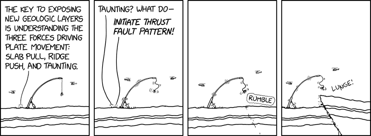
Fault Taunting

XKCD · view →
One of the first things they teach you is to NEVER play with the geology toy over a mantle hotspot.

One of the first things they teach you is to NEVER play with the geology toy over a mantle hotspot.